Nassim Taleb, mathematician and former options trader, is broadly known by having published one of the most iconic books in the field of probability; “The Black Swan: The Impact of the Highly Improbable”. In it, it describes a black swan as an event following three attributes:
1) It is an outlier, as it lies outside the realm of regular expectations.
2) It carries an extreme impact.
3) In spite of its outlier status, human nature makes us concoct explanations for its occurrence after the fact, making it explainable and predictable.
In this short note, we will introduce a way to equip our valuation framework with a powerful tool to take the possibility of these events happening into account: jump diffusion models.
For doing so, we will revisit some of the basic valuation concepts, and then, we will walk through the jump diffusion framework to see how the inclusion of this structure alters the usual approach.
Black-Scholes Valuation Framework
A model is just a simplification of reality. For simplicity, let us suppose that constructing a model is like walking; a sequence of steps. In every additional step, the modeler will always have to consider the trade-off between sticking to reality or, on the contrary, making an unrealistic assumption. One may think that this decision is obvious, but take into account that, sometimes, a faithful representation of the real world may harm the mathematical structure of the model being developed, even leading to making it unsolvable. Another important issue when sticking to reality is the loss of generality, falling into different types of over-fitting. Just like someone walking, you want to arrive to a destination, deviating as little as possible, but knowing that you will finally arrive. Thus, modelers usually take as many assumptions as needed to make a model that can be solved, as general as possible, and loosing the least amount of mathematical robustness.
Most of the valuation models rely on two key assumptions about the markets: they are complete and arbitrage-free. The former means that a derivatives contract can be fully hedged by a specific amount of its underlying, so that we can eliminate the risk. The latter states that there is no way to make a risk-free profit exceeding a theoretical risk-free rate. Fisher Black and Myron Scholes incorporated these assumptions in their paper “The pricing of options and corporate liabilities”, published in 1973 in the Journal of Political Economy. In some Finance degrees, this whole framework is just taught as a formula, but the idea behind is the realization of the aforementioned assumptions (among others). Suppose we have a portfolio composed by the derivatives contract and some amount of the underlying, the latter following a Geometric Brownian Motion:
\begin{align}
\Pi = V(S,t) – \Delta S\\
d\Pi = dV(S,t) + \Delta dS\\
\frac{dS}{S} = \mu dt + \sigma dW_t
\end{align}
where $$W_t \sim N(0, t)$$ By doing some Itô calculus, we end up with the following expression:
\begin{align}
d\Pi = (\frac{dV}{dt} + \frac{1}{2}\sigma^2S^2\frac{dV}{dS^2})dt + (\frac{dV}{dS} – \Delta)dS
\end{align}
In order to erase the risk, we must get rid off the stochastic term (dS):
\begin{align}
\Delta = \frac{dV}{dS}\
d\Pi = (\frac{dV}{dt} + \frac{1}{2}\sigma^2S^2\frac{dV}{dS^2})dt
\end{align}
Additionally, if there is no risk, there cannot be a profit exceeding the risk-free rate. Thus, we end up with the following:
\begin{align}
d\Pi = r\Pi dt = r(V(S,t) – S\frac{dV}{dS})dt\\
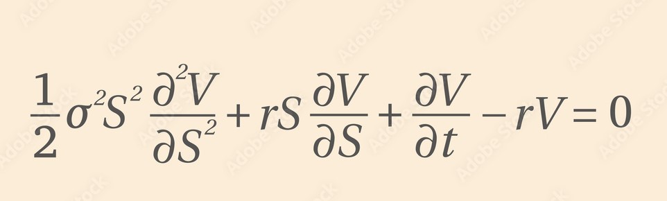
\frac{dV}{dt} + \frac{1}{2}\sigma^2S^2\frac{dV}{dS^2} + rS\frac{dV}{dS} -rV = 0
\end{align}
The equation above, aside of a usual linear parabolic partial differential equation, is one of, if not the most, important developments in Finance. This is because most of the option valuation models are within this framework, adding their own specifications and peculiarities. Now, we will add ours.
A Simple Jump-Diffusion Framework
Robert C. Merton can be considered the founding father of this type of models. In 1976, the Journal of Financial Economics published his paper “Option pricing when underlying stock returns are discontinuous”. He raised the fact that the Black-Scholes option pricing was effective if, and only if, we assume that the underlying stock return dynamics can be described by a stochastic process with a continuous sample path. However, is this true for all assets in the market? Let us look to the 5 day evolution of gold, one of the most traded commodities:
Clearly, these abrupt changes in price (red rectangles) would not have been captured by a GBM-type functional scheme. To be able to account for innovations such as the black swans cited in the introduction, we must equip our SDE describing the dynamics of the underlying with, at least, another term. Merton initially proposed to incorporate a Poisson process, describing its intensity as the probability of receiving an unexpected piece of information which could significantly impact the price of the underlying. Nowadays, researchers are more interested in the use of Hawkes’ processes to model the self-excitation of the order book in a high-frequency trading environment. Since this is just an introductory post, we will focus on defining a simple, yet useful, framework based on the Merton’s original paper.
Consider q as an integer-counting process, defined as the number of times an innovation has arrived in the interval [0,t]. Then, a Poisson process can be described as:
\begin{align} q(0) = 0\\
q(t) = \int_0^t dq \\
dq = \begin{cases}
1 & \mathop{\mathbb{P}} = \lambda dt \\
0 & \mathop{\mathbb{P}} = 1 – \lambda dt
\end{cases} \\
\mathop{\mathbb{P}}[q(t) = n] = exp(-\lambda t)\frac{(\lambda t)^n}{n!}, \forall n \in \mathop{\mathbb{Z^+}}\\
\mathop{\mathbb{E}}[q(t)] = \lambda t\\
\mathop{\mathbb{V}}[q(t)] = \lambda t
\end{align}
With lambda being the intensity (or mean arrival rate) of the Poisson process, i.e. the probability of a jump in the stock price. It is important to remark that, in order to assure that q(t) is a process of this type, increments must be independent. Once equipped with this term, the functional form of the stochastic differential equation would be:
\begin{align}
dS = a(S,t)dt + b(S,t)dW + c(S,t)dq
\end{align}
In the case of a simple stock, we could use the GBM and add the jump term:
\begin{align}
\frac{dS}{S} = \mu dt + \sigma dW + (J-1) dq
\end{align}
Being J the size of the jump. This could be a stochastic process itself, or be calibrated through a data fitting process. A convenient representation is that J follows a log-normal distribution, such that:
\begin{align}
\mathop{\mathbb{E}}[J] = exp(\frac{1}{2}\sigma_J^2)\\
\mathop{\mathbb{V}}[q(t)] = \sigma_J^2
\end{align}
After some Itô calculus, we would arrive to:
\begin{align}
dlog(S) = (\mu – \frac{1}{2}\sigma ^ 2)dt + \sigma dW + (log(J))dq
\end{align}
If you studied Quantitative Finance, this result may be familiar to you. If you didn’t, this is just the development of an exponential martingale, which is commonly used for simulating the stock price when doing option valuation. However, there is one big difference leading us to what comes next. You are right, we do not have the risk free rate, but still the mu term representing the mean of the stock price. Why is that? Consider the same exercise we did in the previous section:
\begin{align}
\Pi = V(S,t) – \Delta S\\
d\Pi = dV(S,t) + \Delta dS\\
\frac{dS}{S} = \mu dt + \sigma dW_t + (J-1)dq
\end{align}
As we have introduced a new source of risk (the Poisson process), the infinitesimal increment of our portfolio value will be different from that of the Black-Scholes framework:
\begin{align}
d\Pi = (\frac{dV}{dt} + \frac{1}{2}\sigma^2S^2\frac{dV}{dS^2})dt + (\frac{dV}{dS} – \Delta)(\mu dt + \sigma dW_t) + (\frac{dV}{dq} – \Delta (J-1)S)dq \\
\frac{dV}{dq} = V(JS,t) – V(S,t)
\end{align}
Now, erasing the risk is not that easy, and, in fact, may not even be possible. Thus, the complete markets hypothesis is being strongly defied. This leads us to take a decision; to completely hedge the diffusion $$\mu dt + \sigma dW_t$$ and forget about the jumps’ risk, or choosing a delta amount such that the risk is minimized, taking the jumps into account. Again, we will stick to the Merton’s approach, but bear in mind that this is not the only solution. The main idea is that, since jumps are a source of idiosyncratic risk, once we hedged for the diffusion, no extra-reward is expected from the market. That is, we still get the risk free rate whether we protect ourselves against the jumps or not. Formally:
\begin{align}
\Delta = \frac{dV}{dS} \\
d\Pi = (\frac{dV}{dt} + \frac{1}{2}\sigma^2S^2\frac{dV}{dS^2})dt + (V(JS,t) – V(S,t) – \Delta (J-1)S)dq \\
\mathop{\mathbb{E}}[d\Pi] = r\Pi dt
\end{align}
Taking into account that:
\begin{align}
\mathop{\mathbb{E}}[(·)dq] = \mathop{\mathbb{E}}[(·) | jump] \lambda dt +
\mathop{\mathbb{E}}[(·)|no-jump] (1 – \lambda) dt
\end{align}
We can summarize the terms that we need in two variables:
\begin{align}
BSE = \frac{dV}{dt} + \frac{1}{2}\sigma^2S^2\frac{dV}{dS^2} + rS\frac{dV}{dS} -rV \\
\mathop{\mathbb{E}}[(·)dq] = \lambda \mathop{\mathbb{E}}[V(JS,t) – V(S,t)] – \lambda \frac{dV}{dS} S \mathop{\mathbb{E}}[J-1]
\end{align}
And taking the integral form of an expectation:
\begin{align}
\mathop{\mathbb{E}}[X] = \int x p(J) dJ
\end{align}
We arrive to the partial integro-differential equation to be solved:
\begin{align}
BSE + \lambda\int_0^\infty V(JS,t) – V(S,t)p(J)dJ = 0
\end{align}
Being p(J) the probability density function of the J (jump) variable. This can still be solved by Monte-Carlo and Finite-Difference schemes (the solution not being local anymore though).
Pros And Cons
Jump diffusion models are powerful tools to value options in a more realistic framework. They allow us to capture jumps in the underlying’s dynamic, something key for contingent claims with a path dependent structure. Also, they provide nice properties regarding the implied distribution of the option being valued. For instance, it can capture extreme implied volatility skews, usually observed in derivatives close to expiration. However, not everything is beautiful. These frameworks usually come with a multi-factor functional form, and, as we saw, may lead to PIDE which, unless we have a nice distribution for the jump component, may be taugh to be solved. This comes along with shaky foundations, such as incomplete markets. Therefore, the big cons with respect to jump diffusion models are the complexity of their structure, and defining the assumptions in such a way that we do not end up with a more unrealistic framework than the starting point, yet being useful.
Personally, I think that these models should be used when dealing with an underlying that clearly reveals a jumping pattern, such that, if calibrated, the jump component will get a sginificant value. This may be the case of some commodities, for which plenty of research has been done about incorporating a jump-diffusion framework, showing empirical positive results. Nevertheless, for assets in which the value of this variable would be negligible, they may not be the best option.
Thank you very much for reading, see you in the next one!