Fractal models are becoming increasingly popular in mathematical finance. However, the way they are explained in the literature is not easy to understand by a non-familiar public. In this short note, I will show the main features of the fractal Brownian Motion (fBM), setting the basis to read a paper containing this family. As an example, I will also introduce how the Black Scholes model can be altered by incorporating fractality to the diffusion.
Introduction
To keep the format of most of the papers about this topic, let us denote a fractal Brownian Motion as \( B_t^H \). H is called the Hurst exponent, a centered Gaussian process lying in the interval (0,1). Then, a fBM satisfies:
\begin{align}
B_0^H = 0\\
\mathop{\mathbb{E}}[B_t^H] = 0\\
\mathop{\mathbb{E}}[B_t^HB_s^H] = \frac{1}{2}[t^{2H} + s^{2H} – |t-s|^{2H}] \quad \forall t,s \ge 0
\end{align}
Note that if H = 0.5, B becomes a standard Brownian Motion (covariance would be the min(s,t)). Therefore, we can say that an fBM is just a generalization of the standard case, accounting for the fact that the covariance of the increments exists, being negative (H<0.5) or positive (H>0.5). In layman terms, this would be translated into having a rougher or a smoother process, respectively.

Once we have the definition, let us delve into 4 basic properties of this kind of stochastic process.
Stationarity of the increments
A stochastic process is said to have stationary increments if its change only depends on the time span of observation, but not on the time when the observation was started.
\begin{align}
B_{t-s}^H \sim N(0, |t-s|^{2H})
\end{align}
Self-Similarity
First of all, let us recall what an homogeneous function is. A function can be considered homogeneous when, if each of the function’s arguments is multiplied by the same scalar, then the function’s value is multiplied by some power of this scalar. The power is called the degree of homogeneity, or simply the degree. We would then say that f(x,y) is homogeneous of degree 2:
\begin{align}
f(x,y) = x^2 + y^2\\
f(tx,ty) = (tx)^2 + (ty)^2 = t^2(x^2+y^2) = t^2f(x,y)
\end{align}
In other words, a process is self-similar if its quantitative properties present symmetry under finer levels of spatial and time scales. In this case, it can be easily derived from the fact that the covariance function of fBM is homogeneous of order 2H.
Long-Range Dependence
Long-range dependence is a term used to describe a pattern where the influence of an event or action persists over a long period of time, even as time goes on.
Imagine you’re throwing a ball against a wall. If you throw it lightly, it might bounce back a few times and then stop. That’s short-range dependence – the effect of your action (throwing the ball) only lasts a short while. But if you throw the ball really hard, it might bounce back and forth many times before finally coming to a stop. That’s long-range dependence – the effect of your action persists over a longer period of time.
In simpler terms, long-range dependence means that something you do, or something that happens, has a lasting impact that continues to affect the situation for quite a while, even as time passes.
Let us define:
\begin{align}
W_n^H = B_n^H – B_{n-1}^H, n\ge1
\end{align}
Then,
\begin{align}
\{W_n^H\}_{n\in\mathop{\mathbb{N}}}
\end{align}
is called the fractional Gaussian noise with Hurst parameter H. It is a stationary sequence normally distributed with unit variance and the covariance function is given by
\begin{align}
\rho_n \sim H(2H-1)n^{2H-2}\\
\rho_n \to 0 \quad as \quad n\to\infty
\end{align}
For long range dependency to occur:
\begin{align}
\sum_{n=1}^\infty\rho_n = \infty
\end{align}
In the case of a standard Brownian Motion, there is not even dependency (p=0). If $H<0.5$, we get a short range dependence, being nice to model sequences with counter-persistence, i.e. it is more likely to decrease in the future if it has been increasing, and vice versa (mean-reverting).
\begin{align}
\rho_n < 0\\
\sum_{n=1}^\infty\rho_n < \infty
\end{align}
On the contrary, if $H > 0.5$, we get that long range dependence. That is, a more “trendy” process, being less likely to break the trend than keep following (momentum).
\begin{align}
\rho_n > 0\\
\sum_{n=1}^\infty\rho_n = \infty
\end{align}
Non-Semimartingale
In essence, a semi-martingale is a mathematical tool used to describe processes that have both predictable patterns and random fluctuations. Formally, a stochastic process X is called a semi-martingale with respect to a filtration \( \mathcal{F}^H_t \) if it admits the following representation:
\begin{align}
X_t = X_0 + M_t + A_t
\end{align}
where M is a local martingale (random), A is a process of locally bounded variation (predictable), and \( X_0 \) is \( \mathcal{F}^H_0 \) measurable (known). This definition implies that any semi-martingale has a locally bounded quadratic variation. That is,
\begin{align}
\pi = {t_0, t_1, …, t_n}\\
v_p(f;\pi) = \sum_{k=1}^n |f(t_k) – f(t_{k-1})|^p\\
v_p(f) = \lim_{|\pi| \to 0}v_p(f;\pi)
\end{align}
exists and is finite. As Rogers shows in his paper “Arbitrage with fractional brownian motion”:
\begin{align}
\lim_{n \to \infty}v_p(B^H;\pi) = \begin{cases}
\infty & pH < 1, \\ \mathop{\mathbb{E}}|B_1^H – B_0^H|^p & pH = 1,\\ 0 & pH > 1
\end{cases}
\end{align}
A standard Brownian Motion (H=0.5) accomplish the condition of semi-martingaelity, but otherwise, it is not accomplished. Why is that? When looking for the quadratic variation in this system, p must be 2. For values lower than 0.5, the result is not even finite. When the Hurst parameter gets values above 0.5, the quadratic variation would have a value of 0. This is finite, but let us assume \( B^H \) is a semi-martingale. Then:
\begin{align}
B_t^H = M_t + A_t\\
\langle B_t^H, B_t^H \rangle = \langle M_t, M_t \rangle = 0
\end{align}
Since a continuous local martingale with zero quadratic variation is constant, a fractal Brownian Motion could be described as a locally bounded variation process.
\begin{align}
M_t = M_0 = 0 \quad a.s.\\
B_t^H = A_t
\end{align}
A locally bounded variation process may have variations that are not integrable over all finite time intervals. For example, it could have discontinuities or jumps occurring frequently enough to prevent the total variation from being integrable. So, while a locally bounded variation process shares some similarities with a semi-martingale in terms of predictability and controlled variation, it may lack the integrability property necessary to be classified as a semi-martingale.
Wrapping up, unless the Hurst parameter is equal to 0.5, then being a standard Brownian Motion, the stochastic process cannot be described as a semi-martingale. This has a terrible impact in terms of mathematical complexity; Itô calculus no-longer applies. At least, as we all know it. Some extensions have been developped, from which Wick calculus stands out, usually denoted with the Wick operator (the little empty diamond: \( \diamond \)). For those wanting to delve into this world, I let you a reference covering most of the Wick-Itô basics: T. E. Duncan, Y. Hu, and B. Pasik-Duncan, “Stochastic calculus for fractional brownian motion i. theory”, SIAM Journal on Control and Optimization.
But don’t worry, for the rest of you just wanting to see how this type of processes could be translated into a day-by-day application, we will now explore how fractals can be implemented in the Black-Scholes framewrok.
Wick Fractional Black-Scholes Model
C. Necula published “Option pricing in a fractional brownian motion environment” in 2002. In this paper, the derivation of the option price formula is almost the same as in the traditional model. Consider two tradable assets in a fractional Black Scholes market with respect to a probability space \( (\Omega, \mathcal{F}^H_t, \mathbb{P}) \), where \( \mathcal{F}^H_t = \sigma({B^H_s} : s \in (0,t)) \):
\begin{align}
dA_t = rA_tdt, A_0 = 1\\
\frac{dS_t}{S_t} = \mu dt + \sigma d^\diamond B^H_t
\end{align}
The explicit solutions for these assets can be represented as:
\begin{align}
A_t = e ^ {rt}\\
S_t = S_0\exp(\mu t + \sigma B^H_t – \frac{1}{2}\sigma ^2 t^{2H})
\end{align}
Then, a Wick self-financing portfolio can be described as:
\begin{align}
V_t = \beta_tA_t + \gamma_tS_t\\
dV_t = \beta_trA_tdt + \gamma_t\mu S_tdt + \sigma S_t d^\diamond B^H_t
\end{align}
Applying the fractional Girsanov’s theorem, it can be found that:
\begin{align}
dV_t = rV_tdt + \sigma \gamma_t S_t d^\diamond \tilde{B}^H_t
\end{align}
where
\begin{align}
\tilde{B}^H_t = B^H_t + \frac{\mu – r}{\sigma}
\end{align}
is a fractional Brownian Motion under an equivalent risk-neutral probability measure \( Q_H \). Thus, under \( Q_H \):
\begin{align}
S_t = S_0\exp(rt + \sigma \tilde{B}^H_t – \frac{1}{2}\sigma ^2 t^{2H})\\
V_0 = e^{-rt}\mathbb{E}^{\mathbb{Q_H}}[V_T]
\end{align}
and
\begin{align}
C(0, S_t) = e^{-r(T-t)}\mathbb{E}^{\mathbb{Q_H}}[max(S_T – K, 0)]\\
C(0, S_t) = S_tN(d^H_+) – Ke^{-r(T-t)}N(d^H_-)\\
d^H_\pm = \frac{ln(\frac{S_t}{K}) + r(T-t) \pm \frac{1}{2}\sigma ^2 (T^{2H} – t^{2H})}{\sigma \sqrt{T^{2H} – t^{2H}}}
\end{align}
It seems that almost nothing changed. It may even look easy, but nothing further from reality. Aside mathematical controversy about Wick operators themselves, think about the time dependence property that we just saw in the previous section. If the Hurst exponent is not 0.5, there is a time dependency that we cannot forget about. In other words, we are valuing path dependent options without taking this path dependency into account, leading to a possibility for arbitrage (see P. Cheridito, “Arbitrage In Fractional Brownian Motion Models”). There are as many models as original ideas to overcome the weaknesses inherent to this framework, but there is not a general consensus about it.
Conclusion
Fractal models are becoming increasingly popular in Mathematical Finance given its flexibility to model the diffusion. They are proving to be useful in many fields, such as volatility modelling and forecasting. However, as we always remark, this comes with an increased mathematical complexity that may be unnecessary for most of the cases, succh as switching from Itô to Wick calculus or having to incorporate time dependency. As modelers, we must always think about the assumptions that we are willing to make and the tradeoff of incorporating such advanced techniques. I hope this post has been useful enough to, finally, being able to read a paper containing these painful diamonds.
Thanks for reading and see you in the next one!